Introduction

When trying to solve problems with computers, it’s generally important to understand both when and why it is that the problem you are trying to solve is hard. This is ostensibly so that you can be smart about trying to solve this problem in practice (maybe don’t spend a million bucks on AWS credits trying to factor large primes, e.g.), but many people (including myself) think that the abstract analysis of problem hardness is interesting in its own right. Regardless of your interest in studying this, hardness of a problem can be measured in a myriad of ways, including:

• computational complexity of a problem (e.g. a problem being NP-hard);
• empirical testing showing that algorithms perform poorly on generic cases of a problem;
• heuristics and lack of a known good algorithm for solving the problem (e.g. the discrete logarithm problem on elliptic curves).

Now, there are some important things to note about when things are determined to be hard:

• problems are often determined to be hard based on the most difficult instances of the problem that could be imagined;
• the hardness of a problem is often based on trying to actually solve it, with no margin of error allowed in the solution.

A classic example along these lines is the knapsack problem which is technically an “NP-complete” problem (tough to solve quickly, easy to verify a solution). However, it is generally considered one of the “easier” NP-complete problems – it can be solved in pseudo-polynomial time. Moreover, there are a number of fast approximation algorithms that, in practice, provide good solutions to the problem that are provably not too far off from the correct answer.

This speaks to two things:

1. The most difficult instances of a problem may be infrequently (or never) realized in “real life”.

2. If I only care about a rough solution to the problem, then I might be able to get away with a faster approximation to a problem solution.

A general framework that lets me talk about solving problems while taking these considerations into account is called property testing, a framework introduced by (Goldreich, Goldwasser, and Ron 1998) and (Rubinfeld and Sudan 1996). I’ll talk more about this paradigm in a future post, but for now, I’m going to dive into a particular, generalizable example where allowing for uncertainty in problem solving allows for gains in computational efficiency.

A problem with graphs

A graph is a collection of nodes that are linked by edges. Graphs are either directed or undirected. In the former case, the edges are assigned a preferred direction (thought of as one node pointing at another node); in the latter, all edges are considered to point in both directions. Here’s an example of an undirected graph of the Seinfeld 2000 characters, where edges represent nodes being friends with one-another:

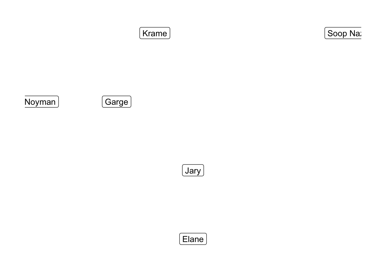
Graphs show up all the time, essentially whenever you are trying to represent relationships between distinct entities. The properties of graphs, then, often correspond to interesting facts about the entities and relationships that are encoded by them. Note that there is a sadder, directed version of the above graph where friendship is not necessarily a symmetric relation. For many, this directed friendship graph is an unfortunate practical model of their relationships.

Connectedness of graphs

One of the most basic things one might ask about a graph is whether or not it is connected, meaning that any two nodes are connected by a path represented by a sequence of edges. The above graph is disconnected by virtue of Soop Naz sitting by himself, and if we removed the link between our boy Krame and his troubled buddy Noyman, it would separate into 3 components.

Connectedness is useful to know about, even if it is a fairly coarse property of graphs to measure – if two nodes in a disconnected graph are not in the same connected component, then this means that there is no sequence of edges that links them to one-another. If the edges represent some relationship (e.g. friendship), then this tells me that the nodes are unrelated to each other, which could be meaningful. In this case, I can tell that Soop Naz is not meaningfully related to anyone, and the ease with which we could disconnect Noyman tells me that he is weakly related to the other members of the graph.

Now, how can I tell if a graph is disconnected? Well, first, I have to deal with actually representing the graph. A standard way of doing this is to consider a graph \(G\) as a function \(N_G\) which for any given node tells me which edges are connected to it:

$$ N_G(v) := \left{ \text{set of edges in } G \text{ with } v \text{ as a starting point } \right} .$$

This is called a “neighborhood” of the node, and being able to obtain the values of \(N_G\) for all nodes in the graph lets me reconstruct the graph itself.

Given this representation of a graph, I can find out if it is disconnected pretty easily, by picking a node \(v\) and doing a breadth-first search (BFS). Starting at \(v\), finding its neighbors by querying \(N_G\), finding the neighbors of those neighbors, etc. will eventually produce all of the nodes that are in the connected component of \(v\). If there are fewer nodes in this component than the total number of nodes in \(G\), then \(G\) is disconnected.

While this is guaranteed to work, the runtime of this algorithm isn’t fantastic – the worst case scenario is when \(G\) is connected, in which case I need to make something like

$$(\text{average number of edges connecting nodes in } G) * (\text{number of nodes in } G) = d N$$

calls to \(N_G\) (or lookups to a list that I am maintaining of nodes visited in the BFS) in order to do the search. If \(G\) is very large and very dense (highly connected), then this could be a lot of operations.

I don’t like doing lots of operations, and I’m not such a stickler for precision. So, what if I don’t demand that I know for sure if I have determined the connectivity of the graph, but rather that I have some reasonable confidence that the graph is connected (ideally with some way to quantify this confidence)?

Phrased another way: can I obtain some probabilistic measurement of the connectedness of \(G\) by doing some more limited search of \(G\), say, by only calling \(N_G\) to find a small number of neighborhoods around a few nodes in \(G\)? You might call this collecting some “local” information around some nodes in \(G\), and then the question becomes “Can I efficiently determine if a graph is probably connected by collecting local information about some nodes?”

At first, you might think that this is impossible. After all, knowing whether or not something is connected is a “global” property of the graph – components can be very large, for example, and without knowing the entire structure of the graph, how will I know if there is not some edge floating around that would connect disparate components of a graph?

The worst-case picture you might have in your head is something like this:

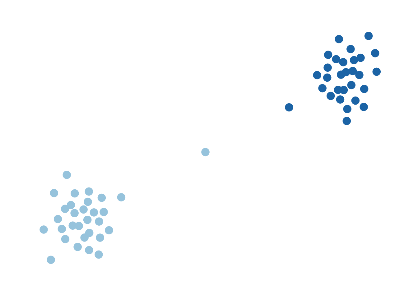
This graph is, of course, connected, but only tenuously so. If I were to remove the edges connected to the single node in the middle (there are only 2), then this thing would become disconnected. In that sense, we can think of this as a graph that is “pretty close” to being disconnected. On the other hand, something like this I would describe as being “far away” from being disconnected:

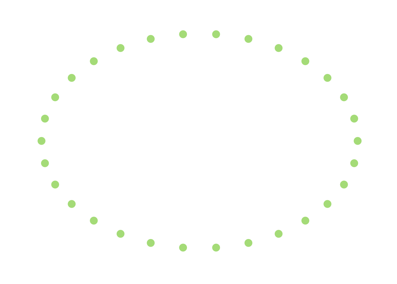
This hints that the worst-case scenario is actually fairly close to being disconnected because of a few scattered edges that are thrown in, and this doesn’t (to me, at least) feel like a very likely situation.

Another, more immediately useful piece of intuition can be obtained by thinking about this from the other side – closeness to connectivity. Take this extremely-disconnected graph:

Thinking about the BFS algorithm I described above, you’ll notice that the search will terminate immediately after I choose a node and see that it has no neighbors, and I would conclude that the graph is disconnected. The reason that this happens is that this graph is very far away from being connected (in that it would take a lot of edge additions to connect it). As a result of this, I’m very likely (certain, in fact) to end my BFS very quickly.

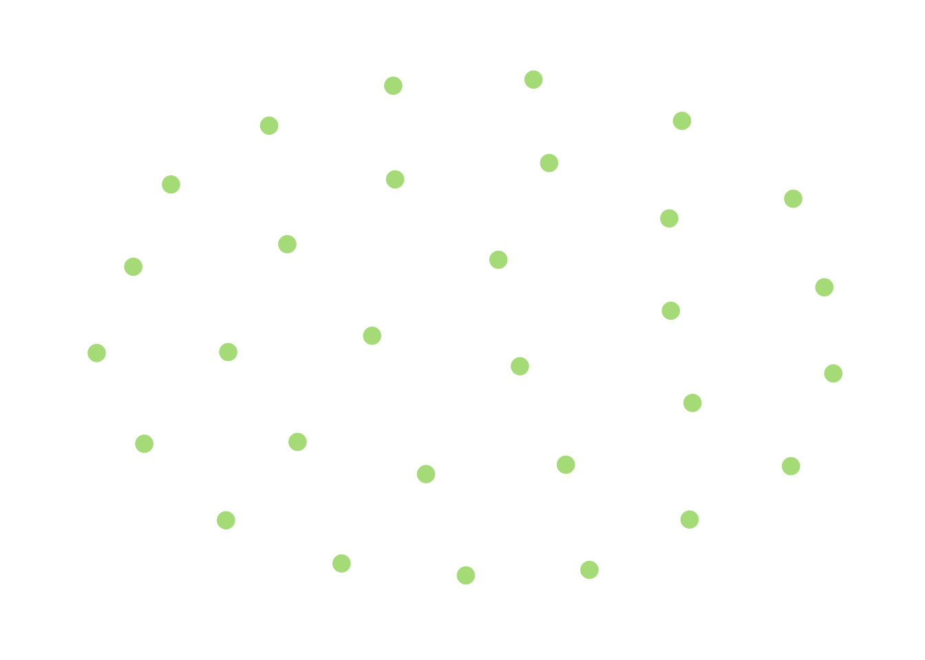
A less trivial example is a modification of the above:

If you imagine moving “closer” to being connected as adding edges to an existing graph to merge components, then this graph is closer to being connected than the previous, completely-disconnected one. However, each component is fairly small, and this suggests that if I demand that \(G\) is far enough away from being connected (in that it would take a lot of edge additions to make it connected) there are going to be a bunch of “small” components.

Moreover, I should be able to find these small components by randomly choosing a bunch of nodes in \(G\) and exploring each of their neighborhoods until I see that it’s bigger than whatever “small” means, at which point I abandon the search and move on to a different random node. If this doesn’t find a small component, then I can guess that \(G\) is connected. This is exactly what happens, and leads to the algorithm described below.

An algorithm

The algorithm I’ll describe relies on the following result from (Goldreich and Ron 1997) which I’ll explain more thoroughly in a subsequent post. For now:

Lemma:

Let \(d \geq 2\), if a graph \(G\) is \(\epsilon\)-far from the class of \(N\)-vertex connected graphs with maximum degree \(d\), then it has at least \(\frac{\epsilon d\cdot N}{8}\) connected components with fewer than \(\frac{8}{\epsilon d}\) vertices.

Ignore what I mean by “$\epsilon$-far” for a moment and think about what this is telling you: if you are given a graph that is far from being connected, then it has a bunch of small components, where “small” is a function of

• how far the graph is from being connected;
• the number of vertices in the graph;
• the bound on the degree of individual nodes in the graph.

This suggests an algorithm for testing if a given graph is “far” from being connected, wherein you pick a bunch of vertices and look for “small” components (you know the biggest they can possibly be) around them. if you fail to find any, then you can guess that the graph is “close” to being connected. to lay it out:

Connectedness algorithm:

1. Randomly select \(m = \frac{16}{\epsilon d}\) vertices in the graph;
2. For each vertex \(v\) perform a breadth first search starting from \(v\) until either \(\frac{8}{\epsilon d}\) vertices have been found or there are no more vertices (in which case you have found a connected component);
3. If any search finds a small connected component, say that the graph is disconnected. If all searches fail, then guess that the graph is connected.

This algorithm:

• runs in \(O\left(\frac{1}{\epsilon^2 d}\right)\) time;
• never rejects a connected graph;
• has at least a 75% chance of being correct when the graph is disconnected and \(\epsilon\)-far from being connected.

This can be made more efficient, and (Goldreich and Ron 1997) provide an algorithm that is \(O\left( \frac{\log^2 (1/(\epsilon d))}{\epsilon}\right)\).

Now, compare this to inspecting the entire graph, which runs in \(O\left(Nd\right)\) time. For \(\epsilon\) small relative to the number of nodes \(N\) (i.e. asking “is \(G\) very close to being connected, relative to the size of \(G\)?”), then you might as well inspect the entire graph. However, if \(N > \frac{16 \log (8/(\epsilon d))}{\epsilon d }\), then you might have a huge gain in computational speed – the algorithm has \(O\left( \frac{\log^2 (1/(\epsilon d))}{\epsilon}\right)\) which is independent of \(N\).

In my view, most remarkable component of this is that it is independent of \(N\). That is, I presented an algorithm which can reliably guess if a graph is disconnected, and runs in a time that is completely independent of how large the graph itself is. The only thing that matters (besides the bound on degree, of course) is how sure you want to be that the graph is actually disconnected, which is encoded by \(\epsilon\).

Next

So far, I’ve talked about determining whether or not a graph is likely to be far away from being connected. There are two directions that I’ll go next:

1. Get into the technicalities of the above algorithm a bit more;
2. Show how this type of thing can generalize.

With regards to the second one: The Lemma is qualitatively like many other results that power property testing algorithms on graphs, and the way that I’d like to think about it for the purposes of generalization is to interpret The Lemma as knowing the possible “shapes” of connected components that could exist.

At the end of the day, the reason that the algorithm works is the knowledge that disconnected graphs that are sufficiently “far enough” away from the set of connected graphs have a bunch of small components floating around, where “small” means that there is a maximum size on the number of vertices in each component.

It is this bound that makes the connectedness algorithm work, allowing us to stop searching around nodes when we have reached the “small component size”. I encourage you to think of “small component size”, then, as a coarse description of the possible shapes that can exist as components of a disconnected graph.

This type of thing generalizes to allow for the approximation of much more complicated properties associated to graphs and topological spaces, where, for example, you could imagine having an idea of “what the possible holes could look like” for a given class of spaces. I’ll get to that in the future, but in the meanwhile, enjoy the new Jery special.

References

Goldreich, Oded, Shari Goldwasser, and Dana Ron. 1998. “Property Testing and Its Connection to Learning and Approximation.” J. ACM 45 (4): 653–750. https://doi.org/10.1145/285055.285060.
Goldreich, Oded, and Dana Ron. 1997. “Property Testing in Bounded Degree Graphs.” In Proceedings of the Twenty-Ninth Annual ACM Symposium on Theory of Computing, 406–15. ACM.
Rubinfeld, R., and M. Sudan. 1996. “Robust Characterizations of Polynomials with Applications to Program Testing.” SIAM Journal on Computing 25 (2): 252–71. https://doi.org/10.1137/S0097539793255151.