The problem

The Survey of Consumer Finances (SCF) is a survey performed by the Federal Reserve every 3 years to gather information about the finances of families in the U.S. It is designed to produce a representative sample of families across various demographics, and so the data can be used to estimate things like distributional properties of income, net worth, savings, etc^[The data that underlies this post is obtained from the 2016 SCF and is viewable here. Don’t take the actual charts here too seriously, though, this is mostly to illustrate visualization techniques and is not a rigorous analysis.].

A cursory analysis of the newly-released 2016 data tells us that the distribution of wealth in the U.S. is incredibly skewed, which leads to difficulties in both data visualization and substantiating claims about the morality of American capitalism. To see why the former is the case, let’s first look at the distribution of wealths in the U.S.

The overall wealth distribution

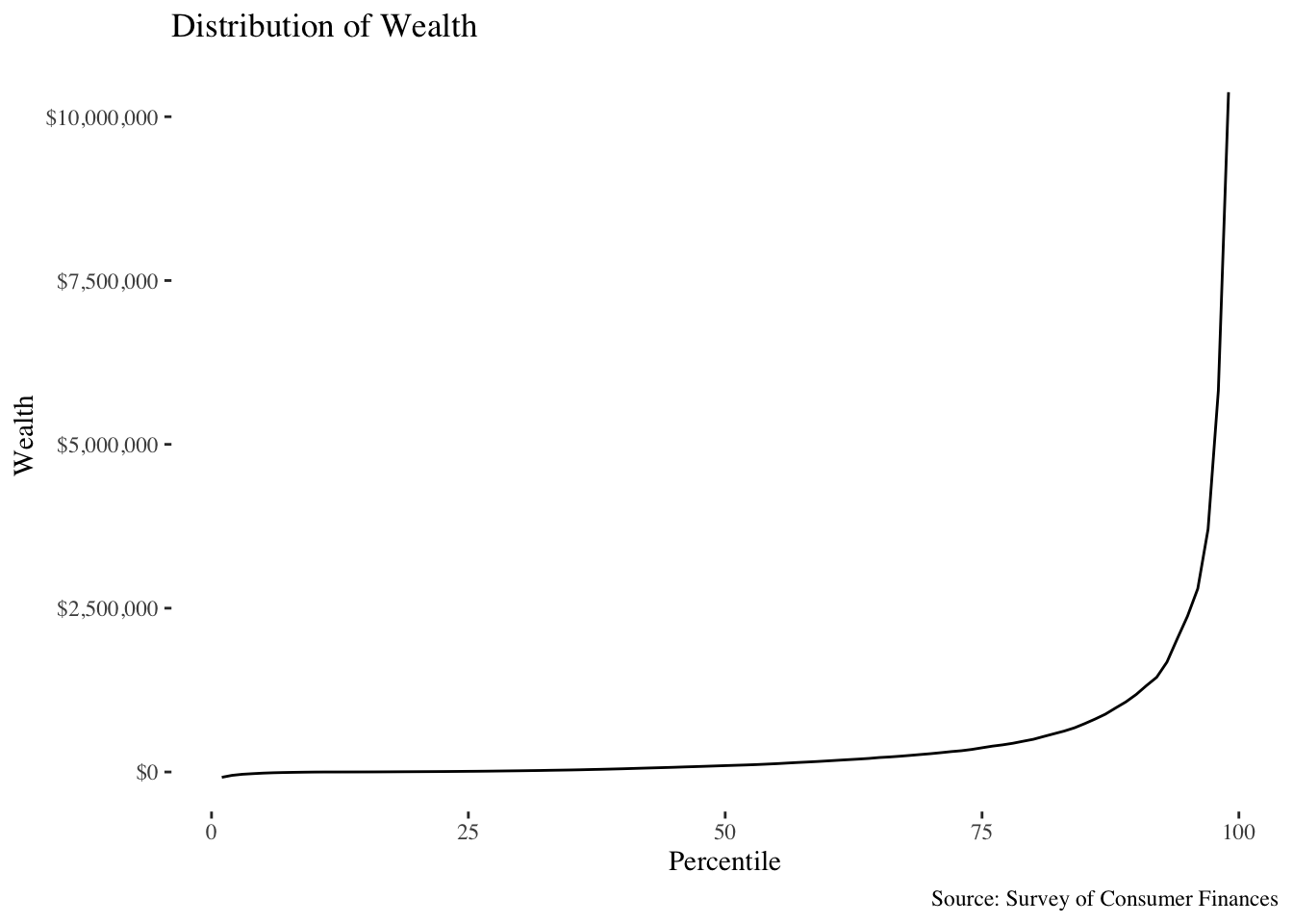
Here’s a percentile plot of the distribution of net worth, which plots the cutoffs for each percentile of net worth against the percentile itself:

A density plot flips this around, and shows the rough likelihood of having a net worth in a specified range. In the following plot, the x-axis represents the net worth, and the y-axis is the probability of having a net worth roughly near the value on the x-axis:

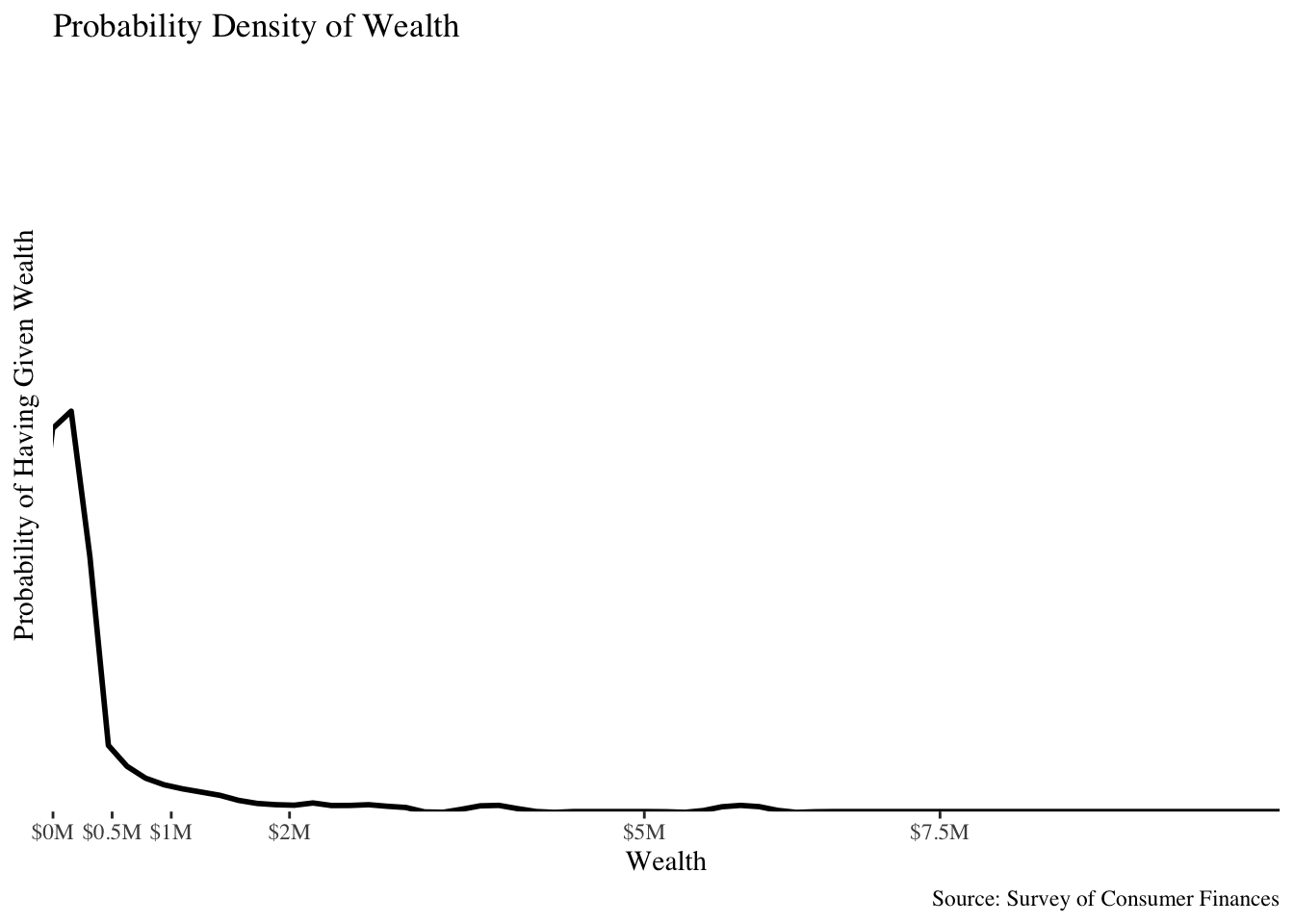
The huge bump on the left corresponds to the near-certainty that you will have a sane net worth (<=$1 million), and the likelihood of you having more wealth becomes almost nil after that point.

This is all to say that there’s a giant “skew” to the distribution of wealth towards a likelihood that you will have a very small (or negative) net worth.

You might already see that this skew becomes a problem if we want to look at the distribution of wealth within a reasonable range – everyone that isn’t super-wealthy gets compressed to a small bump in the density plot, and differences between people who have less than, say, $300,000 are imperceptible in the first percentile plot. This problem becomes more acute when we’re interested in comparing the wealth distributions of subgroups of the overall population.

Wealth distribution across racial groups

The SCF contains information about the racial demographics of the respondents, which is censored to 4 subgroups in the public data release:

• white
• black
• latino/hispanic
• “other”

A good question to ask is: “How are various racial groups doing with respect to one-another, in terms of wealth?”. As we saw above, there is terrible wealth inequality, but is it more terrible for black people?

You might try and compare summary statistics and say things like “The average or median net worth of black families is lower than that of white people.”, which is meaningful, but suffer from some problems (this is true of reporting any single summary statistic of a distribution).

The average is distorted by families that have very large net worths (what’s the average wealth of a room if Bill Gates walks in?) and the median can feel somewhat arbitrary.

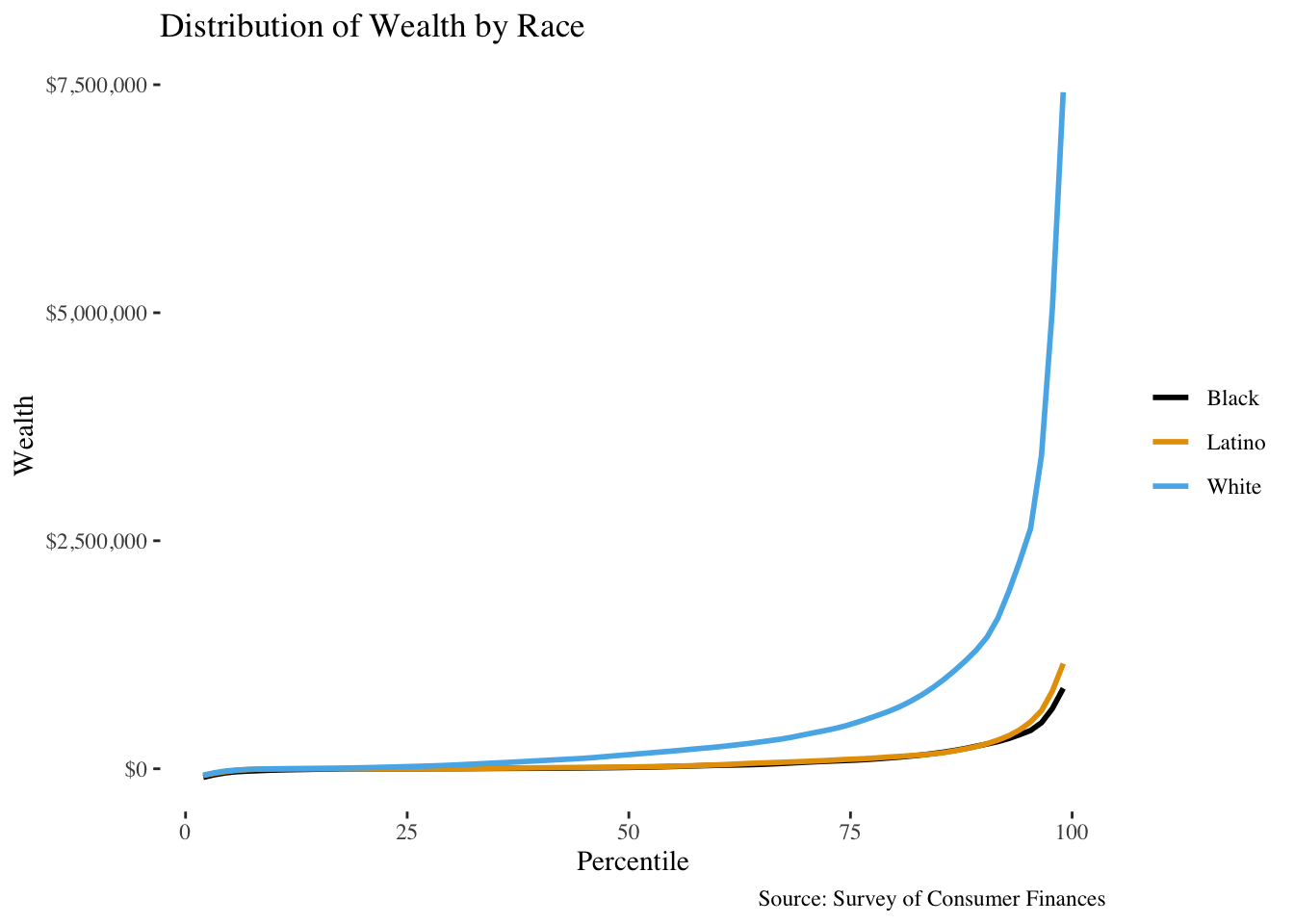
The first thing to try, perhaps, is to plot all of the percentile plots at the same time. This has the same skew problem that we saw before, even though it is a bit informative:

You might try to look at, say, the ratio of racial wealth to white wealth at every percentile:

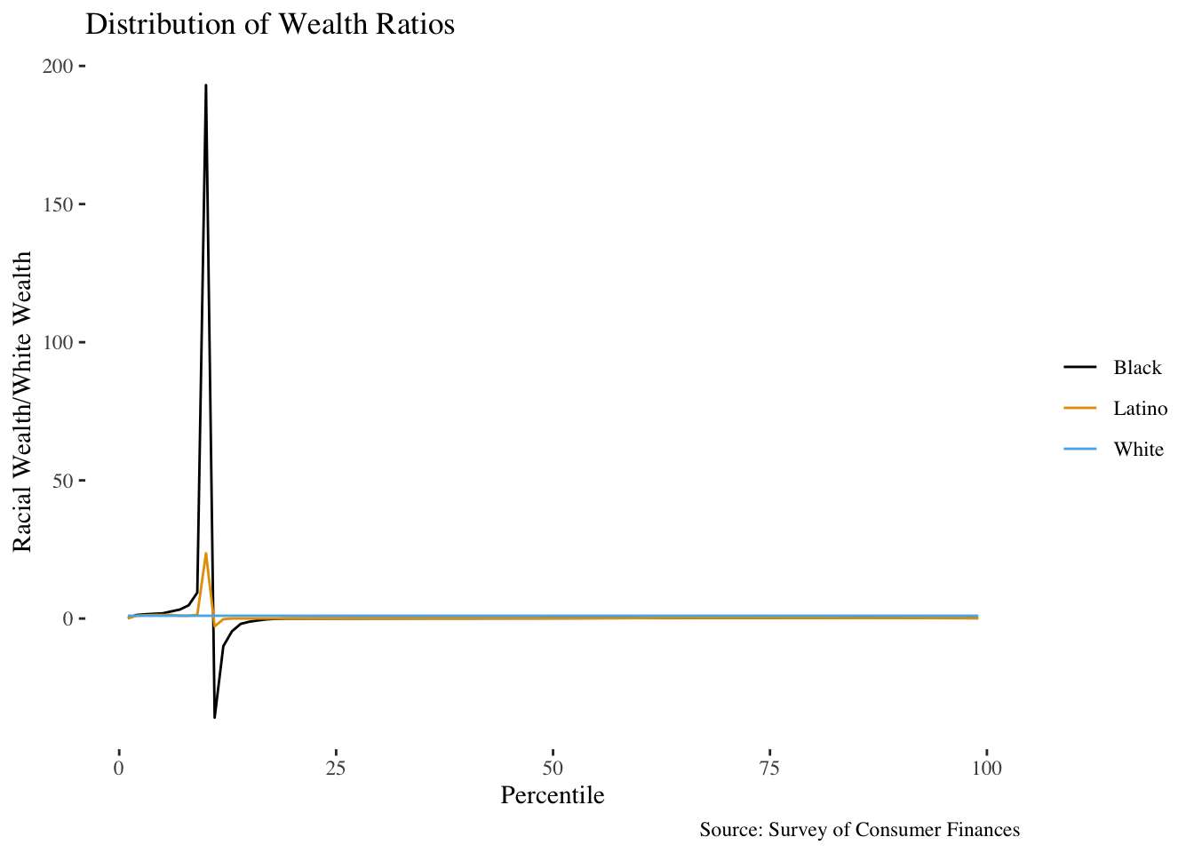
This has both division-by-zero problems and screwy things happening near the lower end of the wealth distribution, where net worths can be negative.

Another naïve alternative is to look at the absolute differences for each percentile:

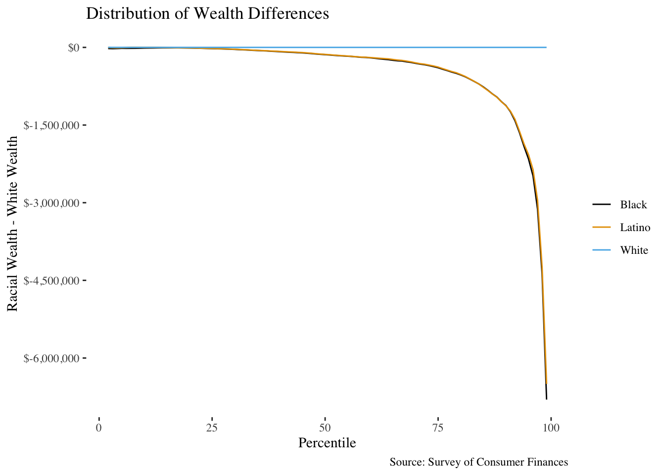
This doesn’t work either, because of the skew in the distribution – the differences are relatively minor at lower wealth than at higher wealth, where, say, a 5% difference in wealth at a net worth of $10 Million would amount to hundreds of thousands of dollars.

So, if we want to display differences in a more “spread out” way, what are we to do?

Some solutions

Fortunately, there are some reasonable solutions to this visualization problem that let us actually see some important differences in the wealth distribution across racial groups. Unfortunately, the results are exactly what you might expect: white people are generally doing far better than blacks or latinos (although there is a case to be made that this relative situation is generally improving).

Q-Q plots

This is the approach taken by Matt Bruenig over at the PPP in this article, which is in line with how many researchers in this field tend to display relative wealth disparities. A Q-Q plot seeks to compare distributions by plotting the quantiles of the distributions against one-another. Below is the simultaneous Q-Q plot of the racial wealth distribution against the overall wealth distribution:

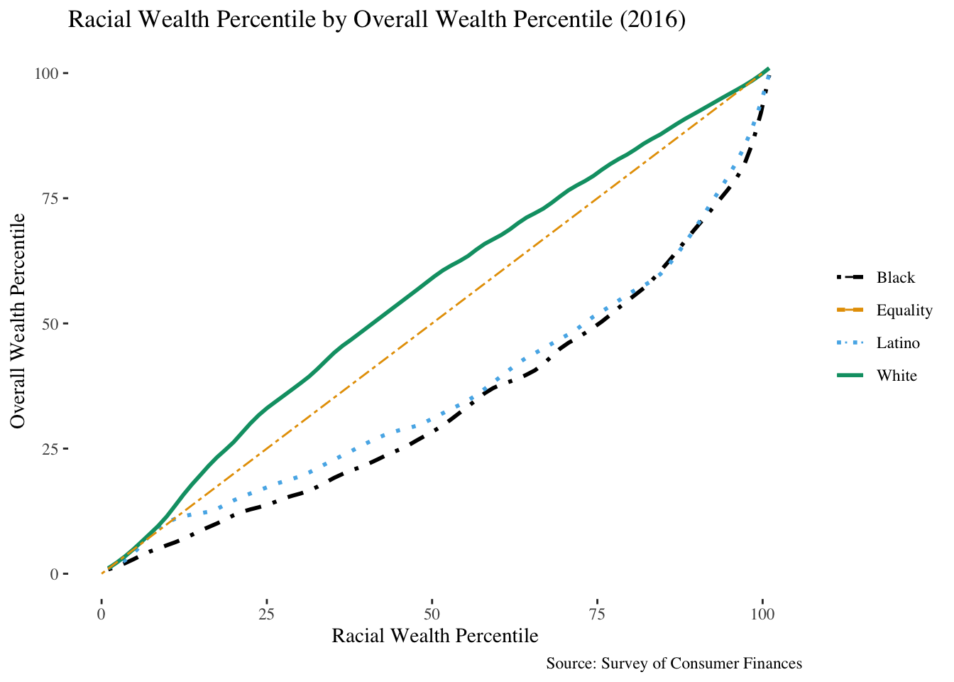
In the above plot, the x-axis is the percentile for the given racial group. This has a corresponding wealth value that is the cutoff for that percentile, and the y-axis represents the percentile in the overall wealth distribution that this wealth value corresponds to. For example, the median income for black families is only in the 28th percentile in the overall wealth distribution, which corresponds to a point \((.50, .28)\) in the above plot on the line corresponding to black families.

The line \(y=x\) corresponds to equality – if there were no difference in the wealth distribution amongst black families and families in general, then the median black income ought to be roughly the same as the overall median income. This is decidedly not the case.

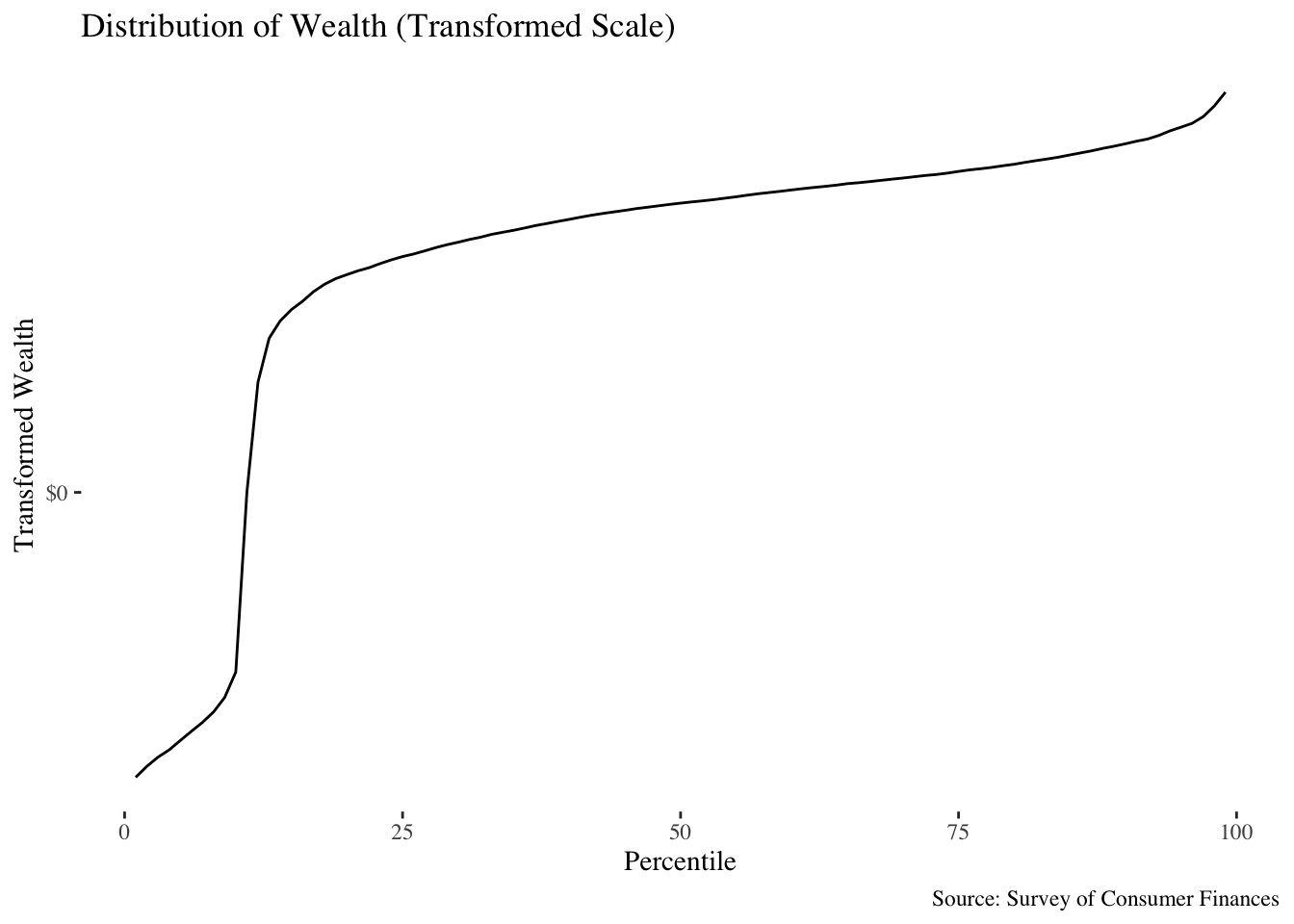
Applying transformations

When dealing with extremely skewed distributions, viewing things on a different scale often helps. A logarithmic transformation, for example, lets us look at orders of magnitude instead of actual values, which has the effect of flattening out the huge, exponentially larger tails of the wealth distribution.

Given that there are negative values of wealth, a logrithm doesn’t quite work (it is undefined for negative values), but something like the inverse hyperbolic sine does the job:

The density plot looks better, as well:

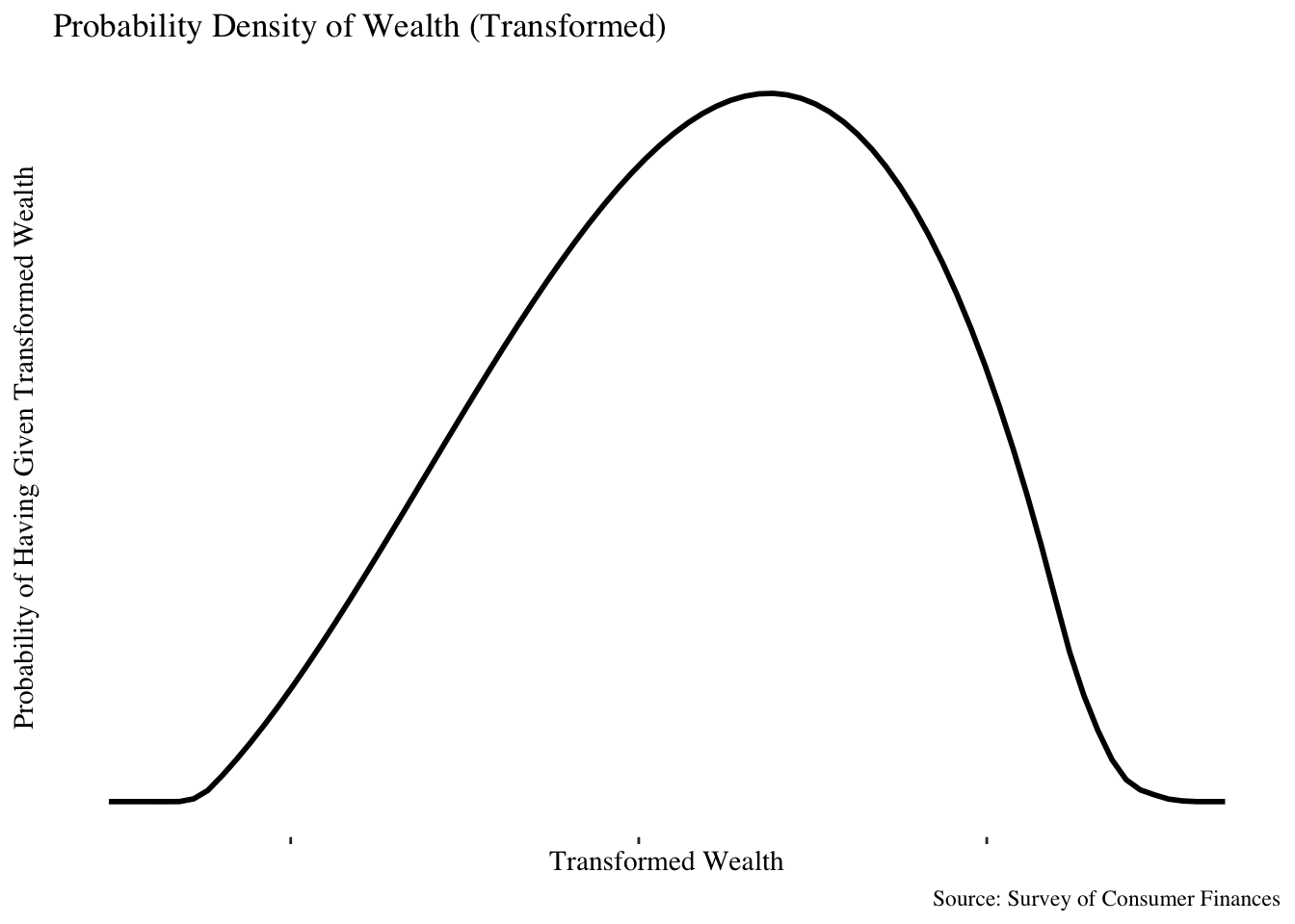
This looks closer to something that is approximately like a normal distribution, which (trust me) is much better. After applying this transformation, the problems around relative comparisons in absolute wealth look much better:

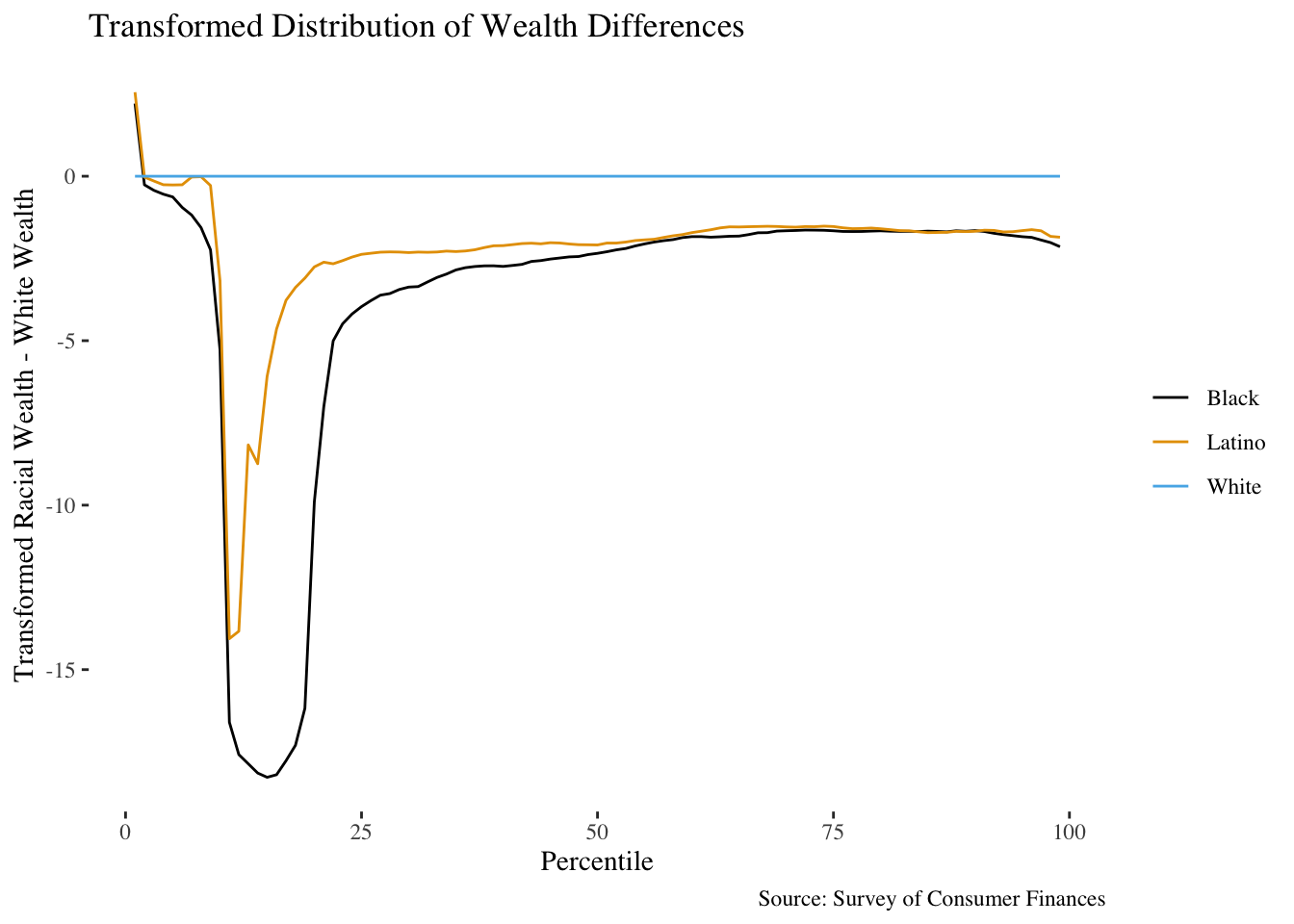
Now here’s a plot that tells us several things!

• Black and latino net worth are consistently lower at every percentile;
• Black net worth is relatively worse than latino income;
• This difference is most acute in the 10-20 percentile range.

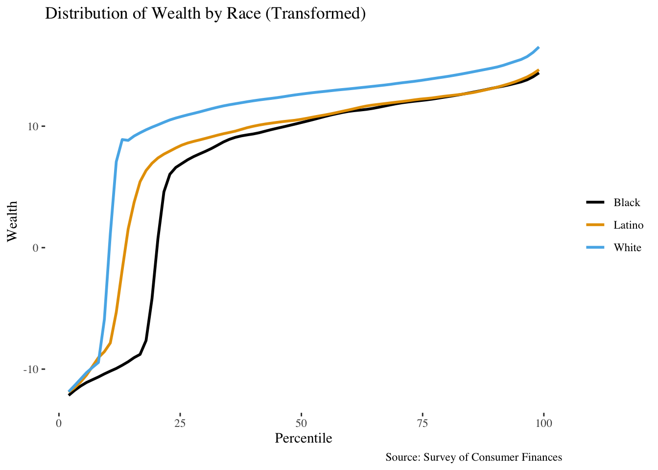
The transformed percentile plots look better as well:

A filled bar chart

This one is a bit strange, but I think it’s worth throwing out there as an option.

The x-axis of this plot is the percentile, and the y-axis is scaled separately so that the positive (negative) values for each percentile sum to 1 (resp. -1) over the different races at each percentile. The positive and negative values are then separately stacked on top of one another, giving you the chart below (I have applied the asinh transformation as well):

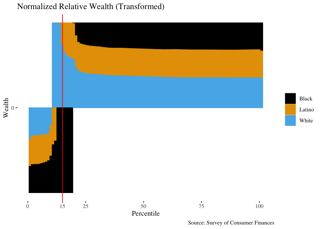
This takes a minute to understand, but I think it provides some decent information. Let’s take a look at an example value, which I’ve marked off with a red line: At the 15th percentile, all of the color below the axis is black. This means that at the 15th percentile, only black families have a negative net worth, while both latino and white families have a positive net worth.

On the other side, we see that the 15th percentile above the line \(y=0\) has a larger proportion corresponding to white families. This tells us that the 15th percentile of white net worth is much larger than the 15th percentile of latino net worth – roughly 75% of all the income at the 15th percentile is taken by white families.

This lets us eyeball:

• Where wealth becomes positive, by looking at where the bars for a given race “flip” to above \(y = 0\);
• The relative proportion of wealths at a given percentile.

A timeless classic

There is, finally, the boxplot. Here’s my take on a Tufte-style minimal boxplot:

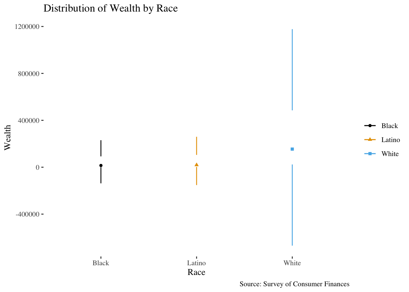
A transformed version of this makes things a bit clearer, as before:

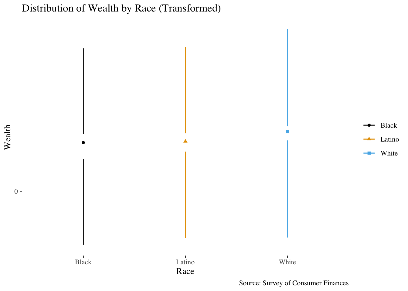
There are also fancier alternatives to this that have their own tradeoffs, like violin plots or pirate plots.

Conclusions

So, what’s the right thing to do? Well, it depends on the audience and personal preference, and every approach has its pros and cons. Here’s my Hot Take:

• The Q-Q plot is a good solution, but requires an explanation of what a Q-Q plot is.
• A transformed plot of the differences may be a bit more approachable – while you lose the interpretability of the values of the y-axis, the structure of the plot itself is familiar to people. You can explain the plot as: “When we plot racial income percentiles on a different scale, here’s what it looks like.”.

I think people will generally be willing to accept the hand-waving around the scaling transformation, especially if getting across the qualitative picture is the overall goal.

• Along those lines, any transformed plot is a decent option if it gets some point across – I think that the transformed percentile plots are good at showing the overall relative differenes in the wealth distributions.
• The stacked bar chart is an option, but it has a lot going on. I personally like it, but it might require a bit too much explanation to be tenable as a general audience graphic.
• Finally, there are classic boxplots. These can also do with variable transformations that allow for visibility.